Homography Transform — Image Processing

Homography Transform | OpevCV

So far what we have discussed is all about manipulating our images in such a way that we detect blobs, segment objects of interest, among others. How about manipulating these images in terms that we transform them from one form to another? Fret not, image processing got you covered! Welcome to a quick discussion on image transformation through the homography matrix.

Homography

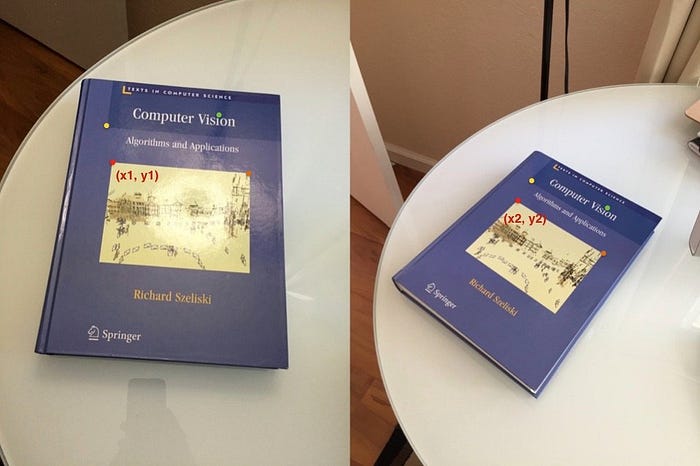
Homography, also referred to as planar homography, is a transformation that is occurring between two planes. In other words, it is a mapping between two planar projections of an image. It is represented by a 3x3 transformation matrix in a homogenous coordinates space. Mathematically, the homograohy matrix is represented as:

How does this look like in a coordinate plane?

As observed in the illustration, the element in an image has its projection to the other image in a homogenous coordinate plane, retaining the same information but in a transformed perspective.

Now, let us implement this in code using Python.

As always, before we can actually do this. The following libraries must be imported:

from skimage.io import imread, imshow
from skimage import transform
import matplotlib.pyplot as plt
import numpy as np

We shall be using multiple images for this article. Download the images by clicking at the link embedded in their captions.

Consider this chess board:

chess = imread('chess.png')
imshow(chess)

Chess Board | Drive (Click here to download)

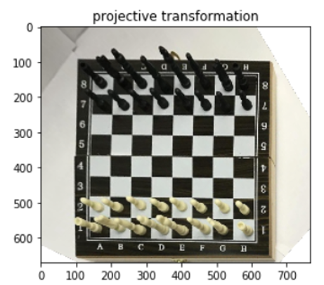
Say you want to instead see a bird’s eye view of the board with its pieces. Is it possible to do that using just the information from the image? Fortunately, yes! And you have to do for this scenario is to locate the corners of the board and set them as your source coordinates. After that, in the same image where you want homography projection to take place, choose your destination coordinate where you would want the transformed image to be displayed.

The code is implemented and is presented below:

#source coordinates
src = np.array([391, 100, 
                14, 271,
                347, 624,
                747, 298,]).reshape((4, 2))
#destination coordinates
src = np.array([100, 100, 
                100, 650,
                650, 650,
                650, 100,]).reshape((4, 2))
#using skimage’s transform module where ‘projective’ is our desired parameter
tform = transform.estimate_transform('projective', src, dst)
tf_img = transform.warp(chess, tform.inverse)
#plotting the transformed image
fig, ax = plt.subplots()
ax.imshow(tf_img)
_ = ax.set_title('projective transformation')

How cool is that? Amazing work! Now that we have done that, how about we do it with another image in mind where the destination points are from that other image? Let us go through this example.

Consider this image, a basketball game.

still2 = imread('still2.png')
imshow(still2)

Basketball Game | Drive (Click here to download)

Say we are interested in transforming half of the court through homography. Can this be done? Let us see.

First things first, identify the source coordinates from the image above (i.e. the corners of the half court). After that, locate our destination coordinates from another image entirely different from the one presented above.

The other image we are talking is presented below:

court = imread('court.png')
plt.imshow(court)

Court | Drive (Click here to download)

Let us see this in action through code:

src_2 = np.array([440, 470,
                  10, 750,
                  1190, 490,
                  1195, 785,]).reshape((4, 2))
dst_2 = np.array([3, 7,
                  3, 506,
                  447, 7,
                  447, 506,]).reshape((4, 2))
fig, ax = plt.subplots(3, 1, figsize=(25, 15))
ax[0].imshow(still2, )
 ax[0].scatter(src_2[:,0], src_2[:,1], c='red', s=30)
 ax[0].set_title('source coordinates')
ax[1].imshow(court)
 ax[1].scatter(dst_2[:,0], dst_2[:,1], c='red', s=30)
 ax[1].set_title('destination coordinates')
dst_2 = dst_2*2 #because image sizes are not the same.
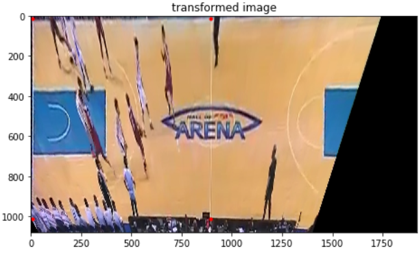
 tform = transform.estimate_transform('projective', src_2, dst_2)tf_img = transform.warp(still2, tform.inverse)
ax[2].imshow(tf_img)
 ax[2].scatter(dst_2[:,0], dst_2[:,1], c='red', s=10)

And there you go, astounding! Transformed image using the homography matrix. Now, we can see the players in another perspective but still retaining the relevant information from the original one.

Very cool, indeed! Now you are now are able to transform images using the homography matrix. Keep posted on my upcoming articles. Fasten you seatbelt and see you in the next article!