Leaf Classification — An Image Processing feature extraction approach to Machine Learning

Alas! The time has come!
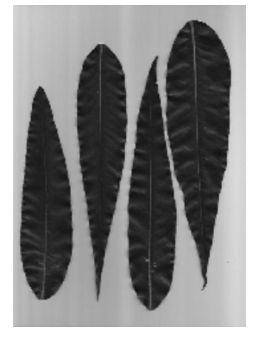
The time has come for us to apply our image processing learnings to an actual machine learning problem. For this blog, let us solve a simple classification problem involving leaves. As a group assignment, our team were provided with a directory containing images of leaves coming from various plants. These images are presented as follows:

As can be seen, there are 5 classes of leaves found in the directory. Hence, we are left with this machine learning problem:
Can we differentiate the various classes of leaves using traditional supervised machine learning methods?
Read until the end of this article in order to find out.
Feature Extraction
The first question you might ask, what features are we going to use in the analysis? In order for machine learning to work, we need to examine features that are common to every leaf category so that the algorithm can then decide what differentiates a leaf over the other. Advancements in deep learning, specifically convolutional neural networks (CNNs), enable us to extract a multitude of features already and obtain high accuracy scores for most of the time. However, since this is a blog about the use of image processing techniques, we shall defer the usage of CNNs in the analysis.
So, if we are not allowed to use CNNs to extract the features from leaves, then how are going to obtain them in the first place? And that is the focus of this blog, using image processing to extract leaf features for machine learning in Python.
As always, the following libraries must be imported to start off the discussion:
 from skimage.io import imshow, imread
 from skimage.color import rgb2gray
 from skimage.filters import threshold_otsu
 from skimage.morphology import closing
 from skimage.measure import label, regionprops, regionprops_table from sklearn.ensemble import GradientBoostingClassifier,
    RandomForestClassifier
 from sklearn.model_selection import train_test_split
 from sklearn.metrics import classification_report from matplotlib import pyplot as plt
 import pandas as pd
 import numpy as np
 from tqdm import tqdm
 import os
To follow along the code implementation, you can download the images through this link: Leaves
Note: Before proceeding, the code implementation for this blog assumes that the directory of leaves is in the same directory as the jupyter notebook. For your information and reference.
Let us take a look at one of our images in grayscale. Run the code below:
 # get the filenames of the leaves under the directory “Leaves”
 image_path_list = os.listdir("Leaves") # looking at the first image
 i = 0
 image_path = image_path_list[i]
 image = rgb2gray(imread("Leaves/"+image_path))
 imshow(image)

Now, let us start extracting the features using skimage ‘region properties’. But before that, we need to preprocess our image, we preprocess the image by binarizing it first using Otsu’s method and cleaned it using the closing morphological operation. The implementation is shown below:
 binary = image < threshold_otsu(image)
 binary = closing(binary)
 imshow(binary)
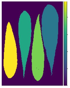
Then, we can label the preprocessed image in preparation for feature extraction.
 label_img = label(binary)
 imshow(label_img)
Finally, let us extract features from the image using region properties. For the purpose of illustration, let us first just consider this image. We will be extracting features from every leaf later on. The code implementation is presented as follows:
table = pd.DataFrame(regionprops_table(label_img, image,
                                       ['convex_area', 'area',
                                        'eccentricity', 'extent',
                                        'inertia_tensor',
                                        'major_axis_length',
                                        'minor_axis_length'])) table['convex_ratio'] = table['area']/table['convex_area']
 table['label'] = image_path[5]
 table
This will give us a dataframe with features we called from regionprops_table function.

Brilliant! It is indeed possible to obtain features. However, that is only for one image. Let us obtain the features for the rest. How to do that? No worries, this blog got you covered. The code implementation on how to do this is provided below:
image_path_list = os.listdir("Leaves")
df = pd.DataFrame()for i in range(len(image_path_list)):

  image_path = image_path_list[i]
  image = rgb2gray(imread("Leaves/"+image_path))
  binary = image < threshold_otsu(image)
  binary = closing(binary)
  label_img = label(binary)

  table = pd.DataFrame(regionprops_table(label_img, image
                          ['convex_area', 'area', 'eccentricity',
                           'extent', 'inertia_tensor',
                           'major_axis_length', 'minor_axis_length',
                           'perimeter', 'solidity', 'image',
                           'orientation', 'moments_central',
                           'moments_hu', 'euler_number',
                           'equivalent_diameter',
                           'mean_intensity', 'bbox']))  table['perimeter_area_ratio'] = table['perimeter']/table['area']  real_images = []
  std = []
  mean = []
  percent25 = []
  percent75 = []  for prop in regionprops(label_img):

      min_row, min_col, max_row, max_col = prop.bbox
      img = image[min_row:max_row,min_col:max_col]
      real_images += [img]
      mean += [np.mean(img)]
      std += [np.std(img)]
      percent25 += [np.percentile(img, 25)]
      percent75 += [np.percentile(img, 75)]  table['real_images'] = real_images
  table['mean_intensity'] = mean
  table['std_intensity'] = std
  table['25th Percentile'] = mean
  table['75th Percentile'] = std
  table['iqr'] = table['75th Percentile'] - table['25th Percentile']  table['label'] = image_path[5]
  df = pd.concat([df, table], axis=0)df.head()

Implementing the code, it has generated a total of 51 features for all the leaves in our images. Now, we are ready for the machine learning implementation. But before that, let us explain some of the features that were extracted to provide context.
We calculated 4 features from region properties.
1. inertia_tensor — This is a tuple representing the tensor of inertia. This relates on the segment’s rotation around its mass.
2. minor_axis_length — This refers to the length of the minor axis or the shorter axis of the segment.
3. solidity — This is just the ratio of the area of the convex hull and the area of the binary image.
4. eccentricity — The eccentricity is the ratio of the focal distance (distance between focal points) over the major axis length.
We also derived these properties from the grayscale raw image segment. All of the features below are just statistics of the grayscale values. IQR is just the difference of the 25th percentile and the 75th percentile.
- 25th Percentile
- 75th Percentile
- mean_intensity
- std_intensity
- IQR
Machine Learning Implementation
Cool Let us proceed to the machine learning implementation.
X = df.drop(columns=['label', 'image', 'real_images'])#features
X = X[['iqr','75th Percentile','inertia_tensor-1-1',
       'std_intensity','mean_intensity','25th Percentile',
       'minor_axis_length', 'solidity', 'eccentricity']]#target
y = df['label']
columns = X.columns#train-test-split
X_train, X_test, y_train, y_test = train_test_split(
X, y, test_size=0.25, random_state=123, stratify=y)
Pick a classifier algorithm. For our team, the best performing one was a gradient boosting classifier. The implementation is as follows:
clf = GradientBoostingClassifier(n_estimators=50, max_depth=3, random_state=123)clf.fit(X_train, y_train)#print confusion matrix of test set
print(classification_report(clf.predict(X_test), y_test))#print accuracy score of the test set
print(f"Test Accuracy: {np.mean(clf.predict(X_test) ==
                             y_test)*100:.2f}%")
Running the algorithm above provides these results:

Findings
The best performing algorithm was the GBM as it has the best test accuracy than all of the classifiers having around 87% test accuracy compared to the 2nd best of 82% from Random Forest. We achived a subtantially high accuracy considering having a PCC of 20% only. Further, the limited number of samples makes the training set be overfitted by the classifiers easily. This can be solved by augmenting the dataset more for generalizability.

And there you have it, an image processing-based approach to a machine learning problem. Great job for reaching this point! See you next time on my next article.
